Introduction to Julia Basics

Introduction

Julia is a dynamically typed compiled programming language developed at MIT for general purpose computing. Julia has a number of interesting features, and is an open source project available under the MIT license.

In this chapter, we will introduce some of the key features of Julia:

• The Julia REPL

• Julia types, functions and syntax

• Writing and Executing Julia Programs

• Using external packages

---

The Julia REPL

You interact with Julia through the Read Evaluate Print Loop (REPL). The REPL allows for quick and easy evaluation of Julia commands; it has a searchable history, tab-completion, many helpful keybindings, and dedicated help and shell modes. The REPL can be started by launching Julia from the Terminal on macOS or by installing Windows Subsystem for Linux and launching Julia from an xterm, or by double-clicking on the Julia executable, or finally by starting Julia from the command line in the terminal of VSCode.

Once the REPL is started, there are four possible modes that it can be in:

• Julian mode: Default mode where commands and expressions are evaluated.

• Help mode: Launches the Julia help system mode where users can view documenation about functions or other Julia features.

• Shell mode: Launches the shell mode which allows users to interact with the operating system shell. For Windows users, Julia’s shell mode does not expose windows shell commands.

• Package mode: Launches the Julia package manager which allows users to add or delete external packages.

Let’s go through each of these modes.

Julian mode

The Julian REPL mode is the default mode of operation; each new line initially starts with the julia> prompt. Julia commands are entered at the prompt and the results are printed to the screen; hitting return or enter after a complete expression has been entered at the prompt will evaluate the entry and show the result of the last expression.

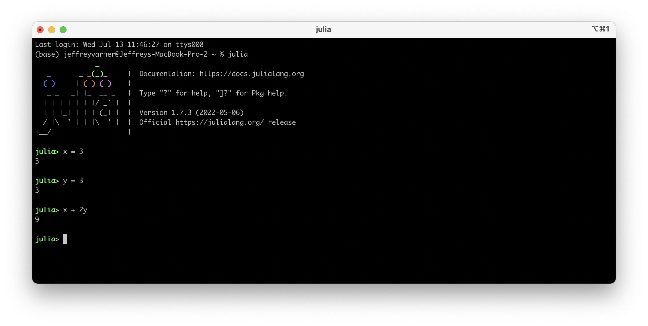
Fig. 3 The Julian REPL mode in the Terminal on macOS.

Fig. 3 shows a case where we enter values for two variables x and yand compute the result of x + 2y.

Help mode

Users enter the help mode by typing a ? character at the prompt. Once in the help mode, which is indicated by the help?> prompt, users can type a command they have a question about (or use TAB for a list of autcomplete possibilities), hit enter and the documentation for that command is displayed.

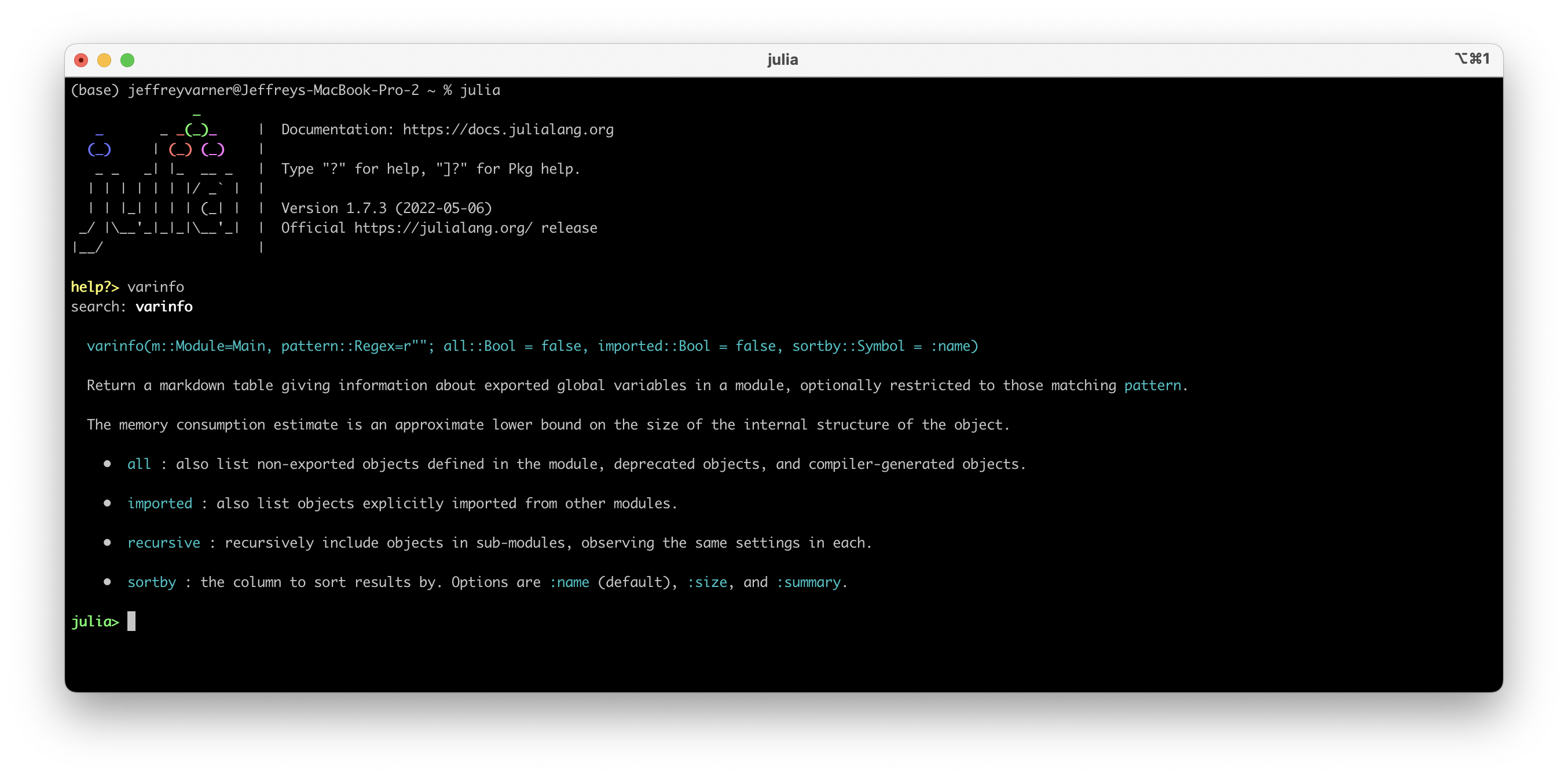
Fig. 4 The help mode in the Terminal on macOS.

Fig. 4 shows the documentation for the varinfo command; varinfo returns a markdown table with information about exported global variables in a module, which (optionally) can be restricted to those matching pattern.

If no search command is entered at the help?> prompt, the user can exit help mode by typing the backspace key (which is the delete key on macOS).

Shell mode

The shell mode is an advanced mode that allows the user to drop down to the operating system shell i.e., a program that exposes an operating system’s services and resources to a user (or other programs).

Users enter the shell mode by typing the ; character at the Julia prompt. Once in shell mode, which is indicated by the shell> prompt, shell commands can be entered and the results displayed.

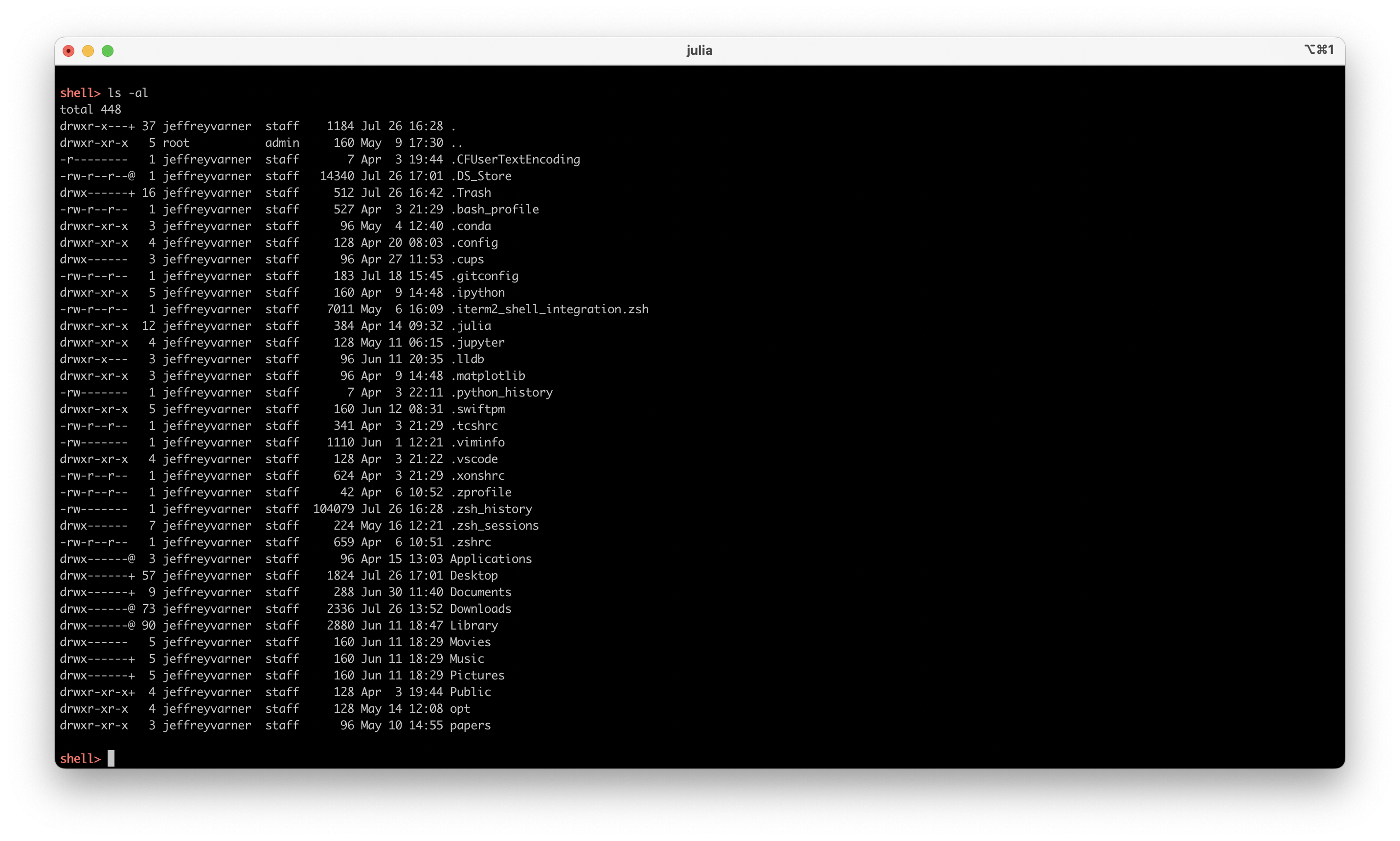
Fig. 5 The shell mode in the Terminal on macOS.

Fig. 5 shows the results of the ls -al shell command; ls -al returns a list of file and directory names in long format for the current directory (my home directory on macOS). To exit shell mode, a user types the backspace key (which is the delete key on macOS).

A list of basic Unix shell commands can be found here.

Package mode

The package mode allows the user to add, delete or update external Julia packages. A user enters package mode by hitting the ] key which brings up the package mode prompt pkg>. At this prompt, users can manage the packages that are installed globally, or in the local project environment.

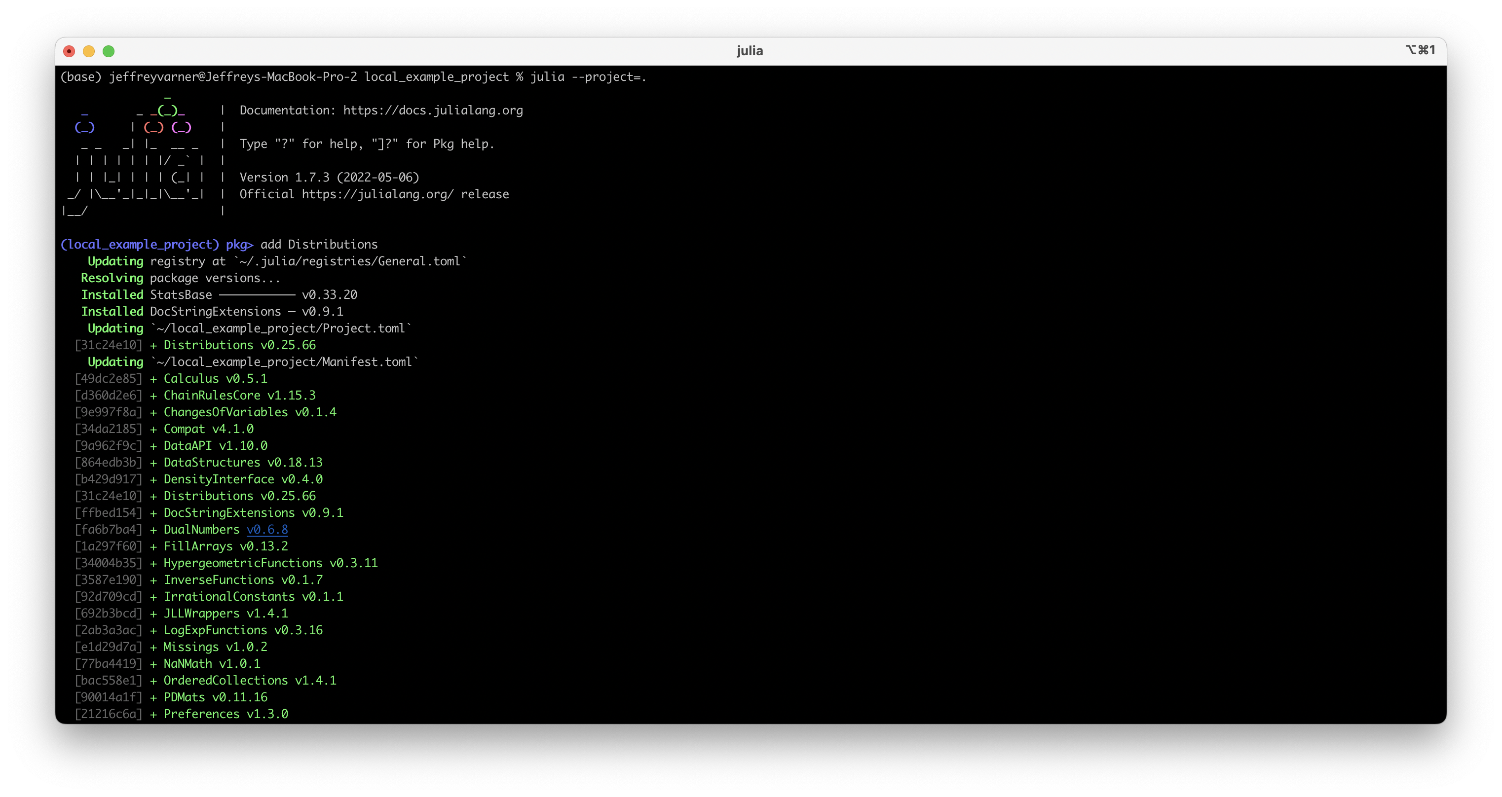
Fig. 6 The package mode in the Terminal on macOS.

The results of the add Distributions command, which installs the Distributions.jl package into the local_example_project project environment is shown in Fig. 6. In addition to adding packages, users can update package versions globally or in the local project environment using the up command; packages can also be deleted using the rm <package> command. A full list of commands for managing packages in package mode can be found here.

To exit package mode, a user types the backspace key (the delete key on macOS).

Loading installed packages into the REPL (or your program) is done with the using or import functions; we discuss what these functions do, and the differences between them, in the Using external packages section.

Julia types, functions and syntax

Julia is a just-in-time compiled language (which gives it a runtime advantage over other popular interpreted languages). However, unlike other languages such as C, Julia code is compiled when you run it; a separate compile step is unnecessary. Thus, Julia gives the convenience and performance of a compiled language without the burden of manual compilation.

Further, Julia is a dynamically-typed language. This means you are not required to declare the type of variables before you use them. Instead, when your Julia code is compiled, the compiler uses sophisticated logic to infer, i.e., guess your data types. However, users can also specify types, potentially lessening the compiler’s burden. Further, many users find codes with the types annotated to be easier to read and maintain; remember, you may be supporting codes for decades, thus, making them easy to understand is critical.

Variable types

Variables are values that you tell your computer to associate with a specific name so that you can later recover or change their values. Variables can be of different types; Julia has an extensive type system. However, in this course we will primarily use floating point numbers, integers and Strings.

In Julia, we do not have to declare a variable name or specify the variable type as in other languages such as C; we can just set the variable, and the compiler will figure out the rest. For example, suppose we wanted to store a floating point value (of type Float64) in the variable x:

# Set the value for the variable x
x = 3.1;

# typeof prints the type of the arg passed in
typeof(x)

Float64

or store an integer (type Int64):

# Set the value for the variable x
x = 1;

# typeof prints the type of the arg passed in
typeof(x)

Int64

or a String:

# Set the value for the variable x
x = "HelloWorld";

# typeof prints the type of the arg passed in
typeof(x)

String

However, in some cases we may want to specify the type of a variable by using the :: annotation, e.g., when composing the list of input arguments or the type of data returned from a function, or the type of items that are stored in a collection of items.

Collections and Data Structures

There are several Collections and Data Structures that come with Julia, for example Arrays, Tuples, Dictionaries and Sets.

In addition to the built-in collection types, a particularly useful data structure is called a DataFrame which is provided by the DataFrames.jl package. We’ll discuss DataFrames in the Working with Data chapter.

Arrays

Arrays are collections that hold ordered lists of items of the same type (typcially). Arrays can be initialized empty (and filled with an arbitraty number of elements) or the number of elements of an Array can be specified when the Array is initialized.

For example, this code block initializes an empty array of Float64 types:

# initialize an empty array of Floats -
x = Array{Float64,1}()

# typeof: prints the type of the arg passed in 
# length: returns number of elements in a 1d Array
typeof(x), length(x)

(Vector{Float64}, 0)

To add elements to an array that has no length, use the push! command:

# initialize an empty array of Floats -
x = Array{Float64,1}()

# add a Float64 -
push!(x,1.32)
push!(x,6.54)

# show the array x -
@show x;

x = [1.32, 6.54]

Alternatively, we can specify the type and number of elements that we need:

# initialize an array of Float64 with 100 elements
# initially each element of the array is of type undef (undefined)
x = Array{Float64,1}(undef,100)

# typeof: prints the type of the arg passed in 
# length: returns number of elements in a 1d Array
typeof(x), length(x)

(Vector{Float64}, 100)

To add elements to an Array with specified dimensions, we can use the Array indexes; the first index is the row number, while the second is the column number of a two-dimensional Array. For example, this code block initializes a 2 x 2 matrix (a two-dimensional array), fills the matrix with ones, and then updates the 1,2-element with a random value:

# initialize a 2 x 2 array A 
A = Array{Float64,2}(undef,2,2)

# fill A with 1's
fill!(A, 1.0)

# update the 1,2 element with a random value -
A[1,2] = rand()

# show A -
@show A;

A = [1.0 0.8073310622535458; 1.0 1.0]

Please read through the Array documentation for a detailed discussion of the properties of Arrays and the various functions that can operate on Arrays.

Tuples

Julia has a built-in data structure called a tuple; a tuple is a fixed-length container that can hold a mixture of values of any type, but cannot be modified i.e., it is immutable once the values have been added to the tuple. In other words, tuples; a tuple are read-only once constructed. Tuples are constructed with commas and parentheses, and can be accessed via indexing:

# initialize a tuple of stuff -
x = (0.0, "hello", 6*7)

# what is held in index 2?
@show x[2];

x[2] = "hello"

Further, you can optionally give the values held in a tuple a name; these types of data structures are called NamedTuples.

# initialize a named tuple of stuff -
x = (firstname="Fred", lastname="Rogers")

# what is the first name?
@show x.firstname;

x.firstname = "Fred"

You can access the values stored in a NamedTuple using dot notation (as shown above). However, because a NamedTuple is just a fancy Tuple, you can also access data through indexing:

# initialize a named tuple of stuff -
x = (firstname="Fred", lastname="Rogers")

# what is the first name?
@show x[1];

x[1] = "Fred"

Dictionaries

One the most useful built-in data structures in Julia is the Dictionary; Dictionaries allow the user to store key => value pairs, where the (key, value) pairs can be anytype.

There are several ways to create Dictionaries in Julia. For example, Dicts can be created by passing pair objects constructed with the => operator to a Dict constructor:

# build a Dict -
d = Dict("A"=>1, "B"=>2)

@show d;

d = Dict("B" => 2, "A" => 1)

This call attempts to infer type information stored in the dictionary from the keys and values, i.e. this example creates a Dict{String, Int64}. However, you can also explicitly specify the types of the key => value pairs by initializing the constructor with type information Dict{KeyType,ValueType}(...):

# build a Dict -
d = Dict{String,Int32}("A"=>1, "B"=>2)

@show typeof(d);

typeof(d) = Dict{String, Int32}

Given a dictionary D, the syntax D[x] returns the value stored in D with key x (if key x exists) or throws an error. On the other hand, a statement like D[x] = y stores the key-value pair x => y in D (replacing any existing value for the key x). Multiple arguments to D[...] are converted to tuples; for example, the syntax D[x,y] is equivalent to D[(x,y)], i.e. it refers to the value with a key equal to the tuple (x,y).

Dictionaries have fast data lookup, insertion, and deletion. Thus, they are ideal for in-memory storage of all kinds of data. However, Dictionaries do not maintain order, i.e., the keys in Dictionary are not ordered. Thus, if the order of data is important then a Dictionary may not by an appropriate data structure. Further, Dictionaries by default are mutable, i.e., they can be changed after they are constructed; this is a good thing most of the time, but care should be taken to regulate changes to dictionaries.

For use cases where data should not be changed, i.e., configuration data or other such applications, an immutable dictionary can be created, see ImmutableDict.

There are many methods for working with Dictionaries, check out the Julia documentation.

Sets

Sets, like arrays, hold a mutable collection of objects. However, unlike an array, the items in a Set must be unqiue. Further, Sets do not maintain order. Thus, a useful mental model for a Set is a sack of unique objects.

Sets are constructured by passing an interable collection of items into the constructor:

# build a set S (notice the brackets)
# We are adding repeated elements, we have two 3's what is going to happen?
S = Set([1, 3, 4, 5, 3]);

@show S;

S = Set([5, 4, 3, 1])

When adding objects to a set, if the object is already present, any repeated objects will not be added. Sets can also be initialized empty, then items added using the push! function:

# build an empty set of type Int
S = Set{Int}();

# add some items to the set S -
push!(S,1);
push!(S,3);
push!(S,5);
push!(S,1); # repeat: will not get added to S

# show the set -
@show S;

S = Set([5, 3, 1])

However, unlike arrays, sets can not be indexed, i.e., there is not an order hence no indexes. Thus, to retrieve an item from a set use the pop! function which removes a random element from the set.

# build a set S -
S = Set([1,2])
println("Output 1: Set S = $(S)")

# remove element -
x = pop!(S)
println("Output 2: what value of x did we get = $(x)")

# show the S -
@show S;

Output 1: Set S = Set([2, 1])
Output 2: what value of x did we get = 2
S = Set([1])

Many functions that work with other collection types, e.g., the length function for arrays, have an equilvent implementation for sets:

# another way to build a set - array comprehension
S = Set{Int}([2i for i = 1:5])

# how many elements?
println("The number of elements of set S = $(length(S))")

The number of elements of set S = 5

Finally, there are several set-specific concepts, which are useful in the context of probability, that have been implemented in Julia. For example, the intersection or union of sets is encoded in the intersect and union functions.

Program Control Flow

Julia provides several tools for program control flow and repeated evaluation; let’s review a few important examples: if statements, while loops and for loops.

If-else-end statements

A common task is to do something if a condition is true, or something else if the condition is false. This task is accomplished with the if-elseif-else-end pattern:

if x < y
    code block-1
elseif x > y
    code block-2
else
    code block-3
end

In the code snippet above, if the conditional expression x < y evaluates to true, then code block-1 is executed; otherwise the conditional expression x > y is evaluated, and if it evaluates to true, the code block-2 is executed; if neither expression is true, the else code block-3 is executed. Let’s see this in action:

# initialize x and y -
x = 10.0
y = 12.0

if x < y
    println("x is less than y")
elseif x > y
    println("x is greater than y")
else
    println("x is equal to y")
end

x is less than y

The elseif and else blocks are optional. Further, as many elseif blocks as needed can be used. The conditional expressions in the if-elseif-else-end construct are evaluated until the first true, then no further conditional expressions (or code blocks) are evaluated. Thus, if we only have one condition to check, e.g., x < y then we can omit the elseif condition:

# initialize x and y -
x = 16.0
y = 2.0

if x < y
    println("x is less than y")
else
    println("x is greater than or equal to y")
end

x is greater than or equal to y

Finally, we may have more multiple statements (or even function calls) in the conditional checks. Suppose we had two complicated conditions that need to be checked to make a decision; perhaps these conditions are computed using two expensive function calls. Let these conditions be a and b.

Logical checks can be chained together with the && and || operators in Julia; these operators correspond to logical and and or operations, respectively. Thus, these operators can check logical and, or logical or conditions. They also have the additional property of short-circuit evaluation: they don’t necessarily evaluate their second argument:

• In the logical and expression a && b, the subexpression b is only evaluated if a evaluates to true.

• In the logical or expression a || b, the subexpression b is only evaluated if a evaluates to false.

While loops

A while loop consists of a control statement and a body:

while statement == true
  body
end

In a while loop, a control statement is evaluated, and as long as the control statement remains true, the code in the body of the while loop is executed. For example:

# declarations -
counter = 1       # loop counter, we start at 1
const limit = 5   # how many times do we want to go around?

# main loop -
while (counter <= limit)

  # body to execute (for now, print info about the counter) -
  delta = limit - counter; # how many more times around?
  println("Counter = $(counter), remaining = $(delta)")

  # update the counter value -
  global counter = counter + 1
end

Counter = 1, remaining = 4
Counter = 2, remaining = 3
Counter = 3, remaining = 2
Counter = 4, remaining = 1
Counter = 5, remaining = 0

In this example, the while loop continues to execute as long the statement \(\text{counter}\leq\text{limit}\) evaluates to true. However, the value of \(\text{counter}\) is updated each pass through the loop. Thus, when the value of \(\text{counter} = 6\), the control statement fails (evaluates to false) and the loop stops.

If the control statement evaluates to false when the while loop is first reached, the body of the while statement is never evaluated.

For loops

The for loop makes repeated evaluation of a code block easier to write; since counting like the while loop is such a common programming task, it can be expressed more concisely with a for loop:

for range
  body
end

where range represent the list of items to iterate over. For example, we can re-write the while loop shown above as a the for loop:

# declarations -
const limit = 5   # how many times do we want to go around?

# main loop -
for i = 1:limit

  # body that is executed (for now, print info about the index) -
  delta = limit - i; # how many more times around?
  println("index i = $(i), remaining = $(delta)")

end

index i = 1, remaining = 4
index i = 2, remaining = 3
index i = 3, remaining = 2
index i = 4, remaining = 1
index i = 5, remaining = 0

where the 1:limit is a range object, which in this case represents the sequence of numbers \(1,2,\dots,\text{limit}\). The for loop iterates through these values, assigning each one to the loop index variable \(i\).

One important difference between the while loop example and the equivlant for loop form is the scope in which variables are visible. If the loop index variable \(i\) has not been introduced previously in another scope, in the for loop form, it is visible only inside of the for loop, and not outside/afterwards. For more information on variable score, see the scope of variables documentation.

Functions

In Julia, a function is an object that maps a tuple of argument values to a return value. Unlike pure mathematical functions, Julia functions can alter their arguments and change the global state of the program. The basic syntax for defining functions in Julia is:

# declare the add function -
function add(x::Float64, y::Float64)::Float64
  return (x+y)
end

# compute the sum of two numbers -
value_1 = add(3.0, 2.0);

# print the resulting value -
println("Value from the add function: $(value_1)")

Value from the add function: 5.0

The add function accepts two arguments x and y (both of type Float64) and returns the sum (also of type Float64). Notice that when we declared the add function, we specified the types of the arguments and the return type using the :: operator.

Thus, if we pass in arguments that are not of the correct type, an error will occur:

# declare the add function -
function add(x::Float64, y::Float64)::Float64
  return (x+y)
end

try 
  
  # compute the sum of two numbers -
  value_1 = add(3.0, "Two");

  # print the resulting value -
  println("Value from the add function: $(value_1)")

catch error
  
  bt = backtrace()
  msg = sprint(showerror, error, bt)
  println(msg)
end

MethodError: no method matching add(::Float64, ::String)
Closest candidates are:
  add(::Float64, !Matched::Float64) at In[22]:2
Stacktrace:
  [1] backtrace()
    @ Base ./error.jl:114
  [2] top-level scope
    @ In[22]:16
  [3] eval
    @ ./boot.jl:368 [inlined]
  [4] include_string(mapexpr::typeof(REPL.softscope), mod::Module, code::String, filename::String)
    @ Base ./loading.jl:1428
  [5] softscope_include_string(m::Module, code::String, filename::String)
    @ SoftGlobalScope ~/.julia/packages/SoftGlobalScope/u4UzH/src/SoftGlobalScope.jl:65
  [6] execute_request(socket::ZMQ.Socket, msg::IJulia.Msg)
    @ IJulia ~/.julia/packages/IJulia/AQu2H/src/execute_request.jl:67
  [7] #invokelatest#2
    @ ./essentials.jl:729 [inlined]
  [8] invokelatest
    @ ./essentials.jl:726 [inlined]
  [9] eventloop(socket::ZMQ.Socket)
    @ IJulia ~/.julia/packages/IJulia/AQu2H/src/eventloop.jl:8
 [10] (::IJulia.var"#15#18")()
    @ IJulia ./task.jl:484

Julia function arguments follow the pass-by-sharing convention, i.e., values are not copied when they are passed to functions. Instead, function arguments act as new variable bindings (new locations that can refer to values), but the values they refer to are identical to the passed values.

Multiple dispatch and generics

In the example above, the add function takes arguments of type Float64, but what if we want to sum arguments of type Int64 or some other numerical format such as Float32 (which is popular in the machine learning community), or a combination of these arguments?

Julia approaches this problem using a technique called multiple dispatch. In particular, program developers can write different versions of the add function that accept different argument types; these different add versions are called methods. At runtime, Julia dynamically determines which method to call based upon the argument types. For example:

# declare the add function that works on Float64
function add(x::Float64, y::Float64)::Float64
  return (x+y)
end

# declare the add function that works on Int64
function add(x::Int64, y::Int64)::Int64
  return (x+y)
end

# Julia determines which version of add to call
value_1 = add(3.0, 2.0);
value_2 = add(2,6)

# print the resulting value -
println("Values from the add methods: value_1 = $(value_1), value_2 = $(value_2)")

Values from the add methods: value_1 = 5.0, value_2 = 8

In this case, the correct version of add is called based on the type of arguments. However, writing different add methods for each argument type (or combination of argument types) would be a burden.

Toward this challenge, Julia has parametric methods in which the argument type itself is variable. In particular, instead of specifying the specific argument type, e.g., Float64 or Int64, we declare rules that generate a set of permissible types that we expect the function can operate on. For example, the parametric add function:

function add(x::T1, y::T2)::Number where {T1, T2 <: Number} 
  return (x+y)
end

specifies that the argument types T1 and T2 are a subtype (defined using the <: operator) of Number, the supertype for all numbers in Julia; thus, we expect the parametric add function to work on any combination of real and complex numbers. This is possible because the + operator that appears in the add function is itself a function with 206 methods (which can be listed using the methods function).

# declare the add function -
function add(x::T1, y::T2)::Number where {T1, T2 <: Number} 
  return (x+y)
end

# Julia determines which version of add to call
value_1 = add(3.0, 2);
value_2 = add(2,6)

# print the resulting values -
println("Values from the add methods: value_1 = $(value_1), value_2 = $(value_2)")

Values from the add methods: value_1 = 5.0, value_2 = 8

Writing and Executing Julia Programs

Julia programs are files with the extension .jl. To load a Julia program contained in Program.jl, the user executes the include command in the REPL where the path to Program.jl is passed in as an argument of type String to the include command.

julia> include("Program.jl")

The code block above loads the code contained in the Program.jl file into the REPL. If Program.jl is an executable script then Program.jl will be executed, otherwise, the variables, data structures and functions encoded in Program.jl will be loaded into the memory of the REPL. To make Program.jl executable, a main method is called (which in turn can load data, call other functions, etc):

function example()

    # stuff happens here
    # ...
end

function main()
    
    # load data 
    # ...

    # call other functions -
    example()

end

# call main method
main()

For example, consider the following executable script:

function example()

    # stuff happens here
    println("A message from inside the example method ... ")
end

function main()
    
    # print a message -
    println("A message from inside the main method ...")

    # call other functions -
    example()
end

# call the main method -
main()

A message from inside the main method ...
A message from inside the example method ... 

The example method is loaded into the REPL memory before the main method (code is parsed by Julia from top to bottom of the file) but example is not executed until is called from the main method.

Using external packages

External packages in Julia are organized as Modules; the basic structure of a module is given by:

module SomeModule

# export, using, import statements are usually here; we discuss these below

include("file1.jl")
include("file2.jl")

end

Thus, modules in Julia are just containers that organize functions, and perhaps user defined types or other data, into a unit. While constructing your own modules is not difficult, it’s beyond the scope of this introduction. For more information on building (and registering) your own modules, please consult the Julia documentation.

Let’s assume that you have used the Package mode to install some external Julia package called Foo.jl. To use that package in your Program.jl (or in the REPL) you’ll need to load Foo.jl module into memory. There are two ways to do that, the using or import functions.

• The using function will load the Foo package and make its exported names available for direct use, i.e., the functions and data contained in the package that are visible are loaded directly into memory for the users of the package. However, names can also be accessed via dot syntax (e.g., Foo.foo to access the name foo), whether exported or not.

• The import function is similar to using with one key exception; import will load the package Foo. However, names from the imported Foo module can only be accessed with dot syntax (e.g., Foo.foo to access the name foo).

Let’s do an example. Suppose we wanted to generate samples from and then visualize a Laplace distribution using Distributions.jl, a Julia package for probability distributions and associated functions, and StatsPlots.jl, a Julia package for statistical visualization. Further, suppose we have already installed Distributions.jl and StatsPlots.jl using the Package mode.

The code block:

# load packages -
using Distributions
using StatsPlots

# Build a Laplace distribution (from the Distributions package)
d = Laplace(0,1); # initialize Laplace distribution with (0,1)

# plot the distribution (from StatsPlots package) -
plot(d,lw=2, label="(0,1)")
xlabel!("Value for x (AU)", fontsize=18)
ylabel!("Laplace(x) proability density (AU)", fontsize=18)

where the Laplace and plot functions are exported from Distributions.jl and StatsPlots.jl, respectively, produces the plot:

Fig. 7 Plot of a Laplace distribution using Distributions.jl and StatsPlots.jl

---

Summary

In this chapter, we introduced some key features of the Julia programming language:

• Working with The Julia REPL

• Julia types, functions and syntax

• Writing and Executing Julia Programs

For more information on Julia, please consult the Julia documentation.